Kaczmarz Algorithm and Related Algorithm Notes

Note: this post contains my study of several papers which are linked here in the blog post. Each of the papers are linked via non-paywalled versions where I could find them at the time of writing. The post also includes some plots to illustrate the variety of approaches to the Kaczmarz algorithm via simulated problem data. Codes to generate the plots are also provided and serve to illustrate the differences via programmatic implementations.

The paper

The Kaczmarz algorithm, row action methods, and statistical learning algorithms is a Contemporary Mathematics, 2018 paper that looks at both Kaczmarz and related problems.

Key points of the paper

1. Relaxations of Kaczmarz can be solved via Hildreth, a variant of Kaczmarz.
2. Projection onto Convex Sets (POCS) where the projections are onto rows of the A matrix (affine hyperplanes).
3. Schwarz iterative method (aka subspace correction method) for solving symmetric positive semidefinite (SPSD) linear systems over separable Hilbert spaces are a generalization of Kaczmarz
4. Randomized Kaczmarz is a special case of SGD w/minibatch size 1 and the objective function is the square of the affine hyperplane.

Note that for the LA approaches you can usually apply Kaczmarz to submatrices given a matrix partition. Partitioned approaches are not discussed in this paper.

Basic Idea of Kaczmarz

You’ve got a system of linear equations (SLE) and you want to solve them,

here \( A \) is a \(rows \times cols \) matrix and \( x \) is a column vector, as is \( b \).

Of course there are several ways in linear algebra (LA) to solve this problem. \( A=LU \) and \( A=QR \) using the LU and the QR decompositions come to mind. Both of those approaches are deterministic as typically presented to students. We will follow a similar approach with Kaczmarz, starting from the deterministic version and progress into randomized etc. versions.

\(x_{k+1} = x_{k} + \alpha_k \frac{b_{i_k} - \langle a_{i_k}, x_{k} \rangle}{\| a_{i_k} \|^2} a_{i_k},\) where \( \alpha_k \in (0, 2) \) for convergence.

Now there is nothing about this that is random as currently written. For an algorithmic procedure we start with an initial guess \( x_0 \) and then update until a convergence criteria is met. This might be a change in \( x_k \) on successive iterates, or a maximum number of iterations. These are two common stopping criteria.

Now we said that this is an SLE but if we instead have inequalities (abbr. SLI) then we handle the solving routinte very similarly

\(c_{k+1} = \textnormal{min} \left\{0, \alpha_k \frac{b_{i_k} - \langle a_{i_k}, x_{k} \rangle}{\| a_{i_k} \|^2}\right\}, x_{k+1} = x_{k} + c_{k+1} a_{i_k}\) where \( \alpha_k \in (0, 2) \) for convergence. The difference here is that if we are on the boundary of the affine hyperplane then we need to stop moving which forces the \( c_k=0 \) for the iteration. If non-zero, then there is some flexibility in movement and the \( x_k \) vector will meander in a meaningful manner.

At this point it may seem like a bunch of formulae and calculations but what is the intuition of why this works?

Why Kaczmarz works

Let’s recall the cosine of the angle between two lines, in LA terms this is written

\(\frac{\langle a, x \rangle}{\| a \| \| x \|} = cosine(\theta),\) where here \( \theta \) is the angle between the two lines, \( a \) and \( x \). That the lines are defined by vectors can be visualized in 2-dimensions where the point in 2 space represents a line emanating from the point \( (0, 0) \) which is often ominously called `the origin’.

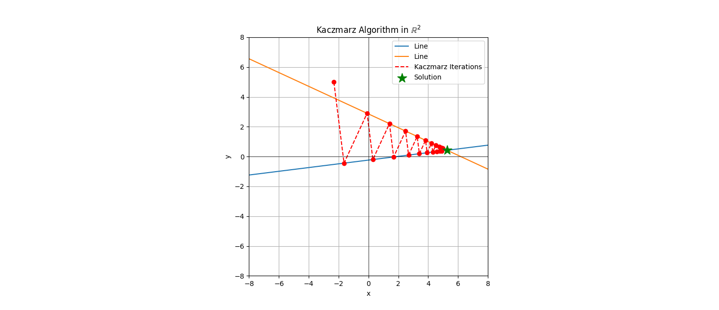
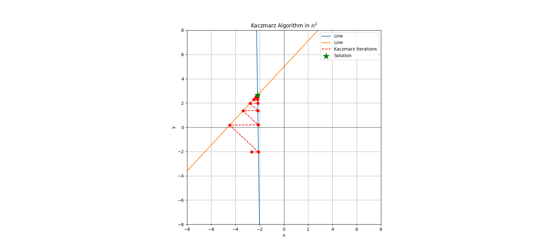
Let’s have some visualization in the Figures 1 & 2.

array of coordinate pairs used to generate the figures for the numerically curious.

# Note this can also be done is num_lines > 2 and the trajectory bounces around a lot more...
# plot is
#Kaczmarx with Ax=b and:
# A = array([[-0.12503767,  1.        ],
#        [ 0.46218237,  1.        ]])
# b = array([-0.23716145,  2.85519088])
# [[-2.31761924  4.98789131]
#  [-1.63867112 -0.44205707]
#  [-0.0945452   2.89888801]
#  [ 0.29299827 -0.20052562]
#  [ 1.40514086  2.20575955]
#  [ 1.68426551 -0.0265648 ]
#  [ 2.48527604  1.7065401 ]
#  [ 2.68631302  0.09872889]
#  [ 3.26323354  1.34698186]
#  [ 3.40802859  0.18897052]
#  [ 3.82355032  1.08801332]
#  [ 3.92783763  0.25396624]
#  [ 4.22711336  0.9014936 ]
#  [ 4.30222534  0.3007788 ]
#  [ 4.51777596  0.76715447]
#  [ 4.57187467  0.33449513]
#  [ 4.72712303  0.67039794]
#  [ 4.76608714  0.358779  ]
#  [ 4.87790335  0.60070994]
#  [ 4.9059669   0.37626924]
#  [ 4.9865015   0.55051779]]



# figure 2 Data
# Kaczmarx with Ax=b and:
# A = array([[66.92575379,  1.        ],
#        [-1.07451305,  1.        ]])
# b = array([-142.79219973,    4.98128477])
# [[-2.66488801 -2.04264369]
#  [-2.10319557 -2.03425092]
#  [-4.47488041  0.17296734]
#  [-2.1366977   0.20790431]
#  [-3.37224101  1.35776778]
#  [-2.15415083  1.3759684 ]
#  [-2.79781446  1.97499661]
#  [-2.16324314  1.98447833]
#  [-2.49856354  2.29654563]
#  [-2.16797984  2.30148519]
#  [-2.34266699  2.4640585 ]
#  [-2.17044745  2.4666318 ]
#  [-2.26145176  2.55132533]
#  [-2.17173296  2.5526659 ]
#  [-2.2191422   2.5967875 ]
#  [-2.17240266  2.59748588]
#  [-2.19710078  2.62047129]
#  [-2.17275154  2.62083512]
#  [-2.18561818  2.6328095 ]
#  [-2.1729333   2.63299904]
#  [-2.17963625  2.63923717]]
# exact solution is: array([-2.17313095,  2.64622719])

To keep things simple I use square 2-dimensional matrices so there are only 2 lines to show. The dashed red line indicates the direction of the movenment of each \( x_k \). These solutions converge on the exact solution, though the progress of the deterministic Kaczmarz decreases with each iteration. You’ll notice that each successive red dot (an \( x_k \) ) is a projection from the previous point orthogonally onto the other line. This behavior holds in higher dimensions as well and if we have a tall matrix instead of a square one we would cycle projections over the 3 or more lines of the matrix, each being an orthogonal projection.

Kaczmarz With Momentum

The paper Randomized Kaczmarz Wwith Geometrically Smoother Momentum is an obvious approach after having visualized the deterministic steps in the plots.

Momentum methods have been around for awhile and the nice thing that they do is take into account these geometries inherent in the space you’re trying to manoever.

The momentum update the authors use is

\(x_{k+1} = x_{k} + \frac{ b_{i_k} - \langle x_k, a_{i_k} \rangle}{\| a_{i_k} \|_2^2} a_{i_k} + M y_k,\) and \(y_{k+1} = \beta y_k + (1-\beta) (x_{k+1} -x_{k}),\) where here \( M \in [0,1] \) and \( \beta \in [0, 1) \). If we set \( \beta = 0 = M \), then we get the usual Kaczmarz algorithm and the \( y_k \) tracks the distance between successive points in the iterations.

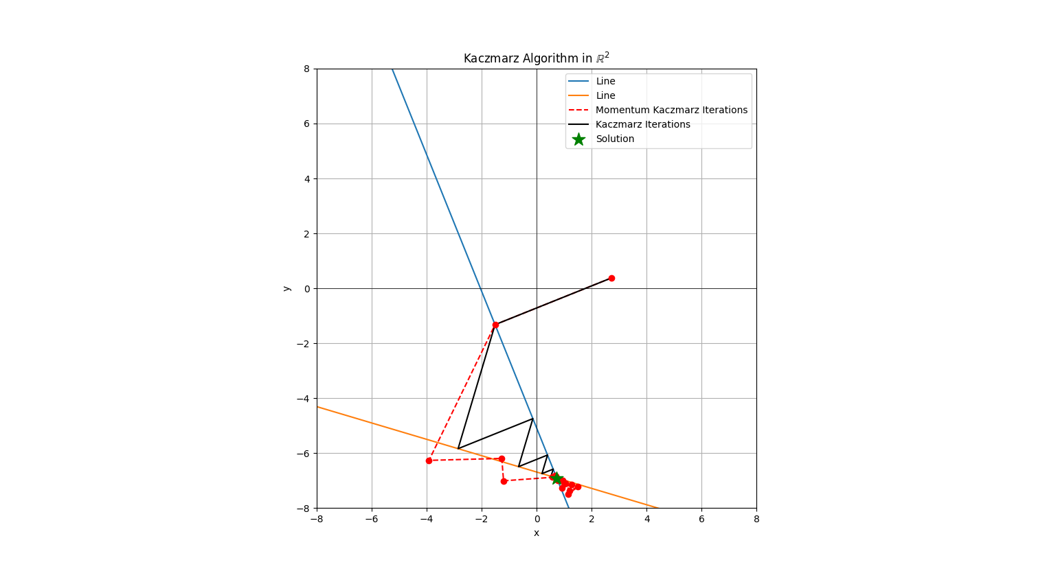
One key difference I’ll point out here is that with a momentum method the steps can exceed the lines which delineate the boundaries in the more standard Kaczmarz steps. Why? The idea is the \( \beta > 0 \) makes the point be a moving point with perhaps constant or non-constant mass behind it as the point moves through the space. The further in the individual steps the point moves, the more momentum is added.

The authors of this work also setup a formulation of Kaczmarz that uses Nesterov Acceleration (NA). NA has 3 equations and I’ll refer you to the paper to read those. They also have a nice theorem that gives quantitive information on the iterations of a randomized NA approach.

In addition, they study the relationship between the eigenspace of the problem and the parameters of the acceleration methods, both Momentum and NA.

The paper is very well written and contains many empirical examples to develop intuitions on the methods.

Code To Generate Simulations For Kaczmarz and Momentum Version

Python code to generate the 2-d Kaczmarz figures

import matplotlib.pyplot as plt
import numpy as np

# Randomly generate an intersection point
intersection = np.random.uniform(-7, 7, 2)

# Randomly generate line angles through the intersection point
num_lines = 2
angles = np.random.uniform(0, np.pi, num_lines)
slopes = np.tan(angles)

# Define the lines: y = m(x - x0) + y0
def line(x, m, x0, y0):
    return m * (x - x0) + y0

# Plot the lines
x_vals = np.linspace(-10, 10, 400)
for m in slopes:
    plt.plot(x_vals, line(x_vals, m, intersection[0], intersection[1]), label=f'Line')

# Kaczmarz algorithm
def kaczmarz(A, b, x0, max_iter=20):
    x = x0
    history = [x0]
    for k in range(max_iter):
        i = k % A.shape[0]
        ai = A[i, :]
        bi = b[i]
        x = x + (bi - np.dot(ai, x)) / np.linalg.norm(ai)**2 * ai
        history.append(x)
    return np.array(history)

# Momentum Kacznarz
def momentum_kaczmarz(A, b, x0, max_iter=20, M=0.5, beta=0.5):
    x = x0
    y = x0 - x0 # always start out with no momentum
    x_history = [x0]
    y_history = [x0]
    for k in range(max_iter):
        i = k % A.shape[0]
        ai = A[i, :]
        bi = b[i]
        x = x + (bi - np.dot(ai, x)) / np.linalg.norm(ai)**2 * ai  +  M*y
        y = beta * y + (1-beta) * (x - x_history[-1])
        x_history.append(x)
        y_history.append(y)
    return np.array(x_history), np.array(y_history)


# suppose now we do a random order on the sam

# Construct A and b from the lines
A = np.column_stack((-slopes, np.ones(num_lines)))
b = -slopes * intersection[0] + intersection[1]

print("Kaczmarx with Ax=b and:")
print(f"A = {A!r}")
print(f"b = {b!r}")
# Initial guess
x0 = np.random.uniform(-5, 5, 2) # this is the first value and is copied into the kaczmarz history

# Run Deterministic Kaczmarz algorithm
history = kaczmarz(A, b, x0, max_iter=20)
if False:
    # Plot the iterations
    plt.scatter(history[:, 0], history[:, 1], color='red', zorder=5)
    plt.plot(history[:, 0], history[:, 1], color='red', linestyle='--', label='Kaczmarz Iterations')

    # Mark the intersection point
    plt.scatter(intersection[0], intersection[1], color='green', marker='*', s=200, label='Solution', zorder=10)

    # Set aspect ratio 1:1
    plt.gca().set_aspect('equal', adjustable='box')

    # these are the X-Y coordinated at each iteration of Kaczmarz

    xy_lim = 8
    print(history)
    exact = np.linalg.inv(A) @ b
    print(f"exact solution is: {exact!r}")
    # Add labels, legend, and grid
    plt.xlabel('x')
    plt.ylabel('y')
    plt.legend()
    plt.grid()
    plt.title('Kaczmarz Algorithm in $\mathbb{R}^2$')
    plt.xlim(-xy_lim, xy_lim)
    plt.ylim(-xy_lim, xy_lim)
    plt.axhline(0, color='black', linewidth=0.5)
    plt.axvline(0, color='black', linewidth=0.5)
    plt.show()


# Run Kaczmarz w/ momentum
x_history, y_history = momentum_kaczmarz(A, b, x0, max_iter=20)
# Plot the iterations
plt.scatter(x_history[:, 0], x_history[:, 1], color='red', zorder=5)
plt.plot(x_history[:, 0], x_history[:, 1], color='red', linestyle='--', label='Momentum Kaczmarz Iterations')
plt.plot(history[:, 0], history[:, 1], color='black', linestyle='-', label='Kaczmarz Iterations')
# Mark the intersection point
plt.scatter(intersection[0], intersection[1], color='green', marker='*', s=200, label='Solution', zorder=10)

# Set aspect ratio 1:1
plt.gca().set_aspect('equal', adjustable='box')

# these are the X-Y coordinated at each iteration of Kaczmarz

xy_lim = 8
print(history)
exact = np.linalg.inv(A) @ b
print(f"exact solution is: {exact!r}")
# Add labels, legend, and grid
plt.xlabel('x')
plt.ylabel('y')
plt.legend()
plt.grid()
plt.title('Kaczmarz Algorithm in $\mathbb{R}^2$')
plt.xlim(-xy_lim, xy_lim)
plt.ylim(-xy_lim, xy_lim)
plt.axhline(0, color='black', linewidth=0.5)
plt.axvline(0, color='black', linewidth=0.5)
plt.show()

I will note that you might need to do some small tweaks to this code if you want to plot the deterministic instead of the momentum overlay-e.g. in the if branch. The code is meant as an illustration not as something super clean.

You might need to modify the source code here a small bit to generate plots like those in the post. You won’t get the exact plots because I forgot to set fixed seeds in the random number generators. Play around with the code a bit though, you’ll see similar figures as you execute the code.

Greedy Kaczmard

The paper Convergence Rates for Greedy Kaczmarz Algorithms, and Faster Randomized Kaczmarz Rules Using the Orthogonality Graph

Looks at two row selection rules that are deterministic but greedy and update as we move through the space. In the simple Kaczmarz algorithm we update (project) onto rows {0, 1, …, # rows - 1} successively. We then go back and do the full pass again and again until stopping criteria are met.

With the greedy approach they use the following rules

\(i_k = \textnormal{argmax}_i \| a_i^Tx_k - b_i \| \ \ \textnormal{(MR)},\) or \(i_k = \textnormal{argmax}_i \| \frac{a_i^Tx_k - b_i}{\| a_i \|} \| \ \ \textnormal{(MD)},\) where the MR and MD are for maximal residual and maximal distance, the distance being between \( x_k \) and \( x_{k+1} \). The thing I like about these row selection rules is that they learn as the algorithm progresses. This learning comes from the inclusion of the \( x_k \) values in the calculation. The tradeoff is that the learning comes at a cost, for each update when we learn new row entering residuals or distances, we incur a search/sortation cost of \( \mathcal{O}(r) \) where \( r \) is the number of rows in the matrix \( A \). This is the cost of looking for the new max residual or max distance row. This is because the state in the solution space changes so that you must recalculate all of the residuals or distances change when you update.

This paper also mentions that SLI can be solved with the greedy approach too. By now we know that this is pretty straightforward. One interesting note they mention is that you can do any sort of norm optimization with a constraint with the SLI approach. The paper mentions using the SLI with a binary search over \( \tau \) to solve

\(\textnormal{min}_{x} f(x) = || Ax - b ||_1 + \lambda || x ||_1, \lambda \geq 0.\) And using \( f(x) \leq \tau \) where we vary \( \tau \) on each iteration, basically transforming the L_1 constrained L_1 optimization problem into a univariate binary search and using the Kaczmarz as a subroutine.

Python code to generate the 2-d Kaczmarz figures

## scratch code for greedy Kaczmarz


import matplotlib.pyplot as plt
import numpy as np


# Kaczmarz algorithm
def kaczmarz(A, b, x0, max_iter=20):
    x = x0
    history = [x0]
    for k in range(max_iter):
        i = k % A.shape[0]
        ai = A[i, :]
        bi = b[i]
        x = x + (bi - np.dot(ai, x)) / np.linalg.norm(ai)**2 * ai
        history.append(x)
    return np.array(history)

# Greedy-Kaczmarz algorithm
from heapq import *

def greedy_kaczmarz(A, b, x0, max_iter=20, max_residual=True):
    x = x0
    x_history = [x0]
    num_rows = A.shape[0]
    rows = [(-abs(np.dot(A[row,:], x) - b[row]).item(), row) for row in range(num_rows)]
    row_history = [rows]
    heapify(rows)
    for k in range(max_iter):
        i = rows[0][1] # row of largest abs residual
        ai = A[i, :]
        bi = b[i]
        x = x + (bi - np.dot(ai, x)) / np.linalg.norm(ai)**2 * ai
        if max_residual:
            # this corresponds to max distance rule (eqn 3) in paper
            rows = [(-abs(np.dot(A[row,:], x) - b[row]).item(), row) for row in range(num_rows)]
        else:
            # this corresponds to max distance rule (eqn 4) in paper
            rows = [(-abs(np.dot(A[row,:], x) - b[row]).item() / np.linalg.norm(A[row,:], ord=2), row) for row in range(num_rows)]
        heapify(rows)
        x_history.append(x)
        row_history.append(rows)
    return np.array(x_history), row_history


# Define the lines: y = m(x - x0) + y0
def line(x, m, x0, y0):
    return m * (x - x0) + y0

# Randomly generate an intersection point
intersection = np.random.uniform(-7, 7, 2)

# Randomly generate line angles through the intersection point
num_lines = 3
angles = np.random.uniform(0, np.pi, num_lines)
slopes = np.tan(angles)

A = np.column_stack((-slopes, np.ones(num_lines)))
b = -slopes * intersection[0] + intersection[1]

# Plot the lines
x_vals = np.linspace(-10, 10, 400)
for m in slopes:# Construct A and b from the lines
    plt.plot(x_vals, line(x_vals, m, intersection[0], intersection[1]), label=f'Constraint Line')


# Initial starting guess
x0 = np.random.uniform(-5, 5, 2) # this is the first value and is copied into the kaczmarz history

# Run Deterministic Kaczmarz algorithm
history = kaczmarz(A, b, x0, max_iter=20)
# Run Kaczmarz w/greedy choice
## NOTE: change `max_residual=False` to `max_residual=True` to toggle the two greedy choices
## from the greedy Kaczmarz paper
max_residual=False
x_history, row_history = greedy_kaczmarz(A, b, x0, max_iter=20, max_residual=max_residual)
# Plot the iterations
plt.plot(history[:, 0], history[:, 1], color='red', linestyle='--', label='Kaczmarz Iterations')
plt.scatter(x_history[:, 0], x_history[:, 1], color='black', zorder=5)
plt.plot(x_history[:, 0], x_history[:, 1], color='black', linestyle='--', label='Greedy Kaczmarz Iterations')
# Mark the intersection point
plt.scatter(intersection[0], intersection[1], color='green', marker='*', s=200, label='Solution', zorder=10)

# Set aspect ratio 1:1
plt.gca().set_aspect('equal', adjustable='box')
#plt.plot(x_vals, line(x_vals, m, intersection[0], intersection[1]), label=f')
#plt.plot(x_vals, line(x_vals, m, intersection[0], intersection[1]), label=f'Line', color="purple")

# these are the X-Y coordinated at each iteration of Kaczmarz

xy_lim = 8
# exact = np.linalg.inv(A) @ b
# print(f"exact solution is: {exact!r}")
# Add labels, legend, and grid
plt.xlabel('x')
plt.ylabel('y')
plt.legend(bbox_to_anchor=(1.05, 1), loc='upper left') # puts the legend outside of plot-top left
plt.grid()
if max_residual:
	plt.title('Kaczmarz vs Greedy Max Residual Algorithm in $\mathbb{R}^2$')
else:
	plt.title('Kaczmarz vs Greedy Max Distance Algorithm in $\mathbb{R}^2$')
plt.xlim(-xy_lim, xy_lim)
plt.ylim(-xy_lim, xy_lim)
plt.axhline(0, color='black', linewidth=0.5)
plt.axvline(0, color='black', linewidth=0.5)
plt.show()

Here are two plots of the Minimal Residual (MR) method and Minimal Distance (MD) methods take from the paper. The figures overlay the same Kaczmarz iterations from the simple approach against the two greedy methods.

From the figures you can see that steps which are longer are selected as the projection steps. Once you are in a range close to the solution point the greedy choice seems to matter less unless you need a lot of precision for the vector entries.

These two greedy methods vary slightly in terms of the order or projections.

For these plots you’ll notice I generated 3 rows rather than 2 for the 2 dimensional examples, the reason is to inject some variation into the selection of the rows, if there were only 2 rows then the projects would still alternate. I could’ve made the simulations have more the 3 rows but I wanted the figures to be relatively clear in terms of illustrating the behavior for the greedy Kaczmarc variants.

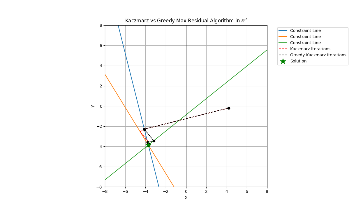
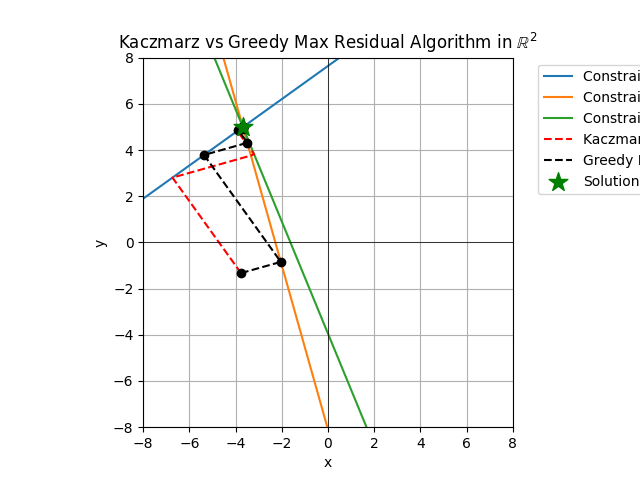
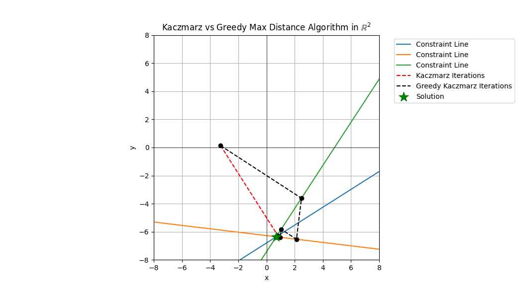
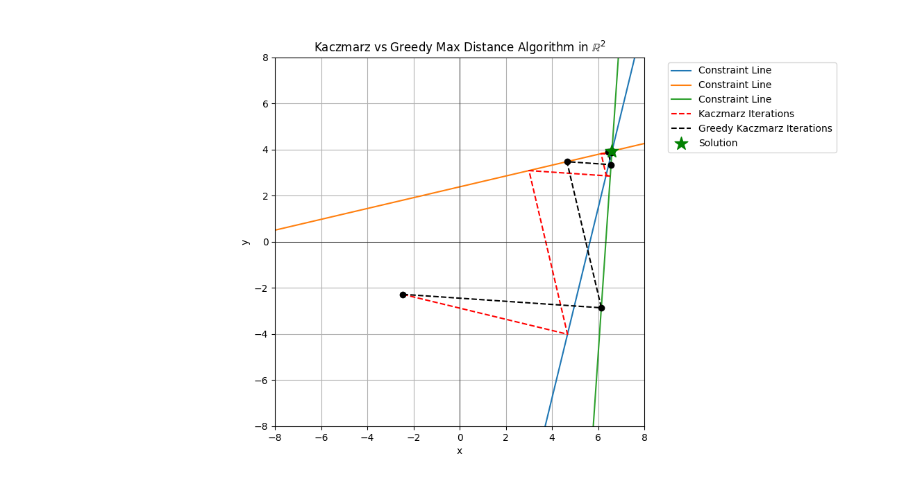
In both pairs of plots we see that often the trajectory of the simple Kaczmarz and the greedy variant follow similar patterns with perhaps one or two steps differening. These steps which differ, if early enough in the iteration process can have a large difference on the solution. Therefore, if you have an application where something close enough will suffice and the close enough is somewhat flexible, these greedy methods are worth looking into further.

Application To GUI Layouts

The manuscript by gives several applications. One that I think is cool is to GUI layouts with hierarchies. You can think of CSS flexbox as an example but the Auckland model is more layered IIUC.

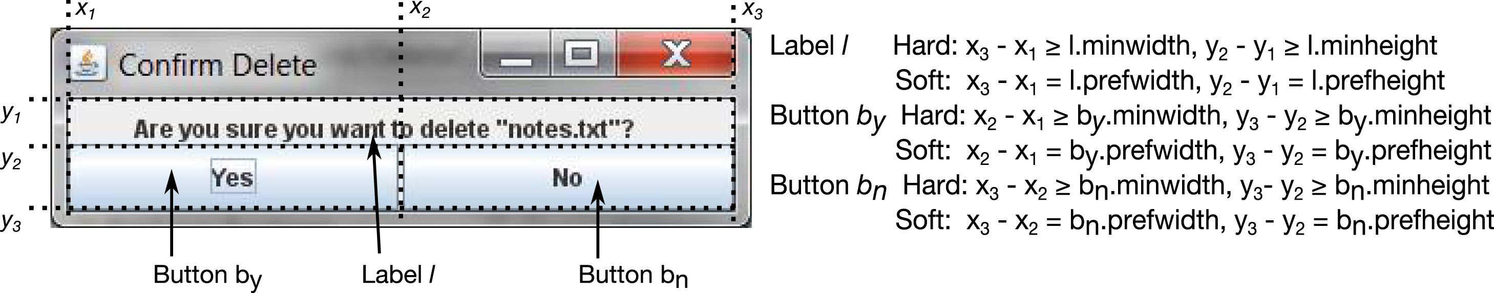
The figure gives you an idea of the mixture of hard/equality vs soft/inequality constraints that go into setting up a visualization layout of widgets.

The hierarchy in the Auckland layout model is a list of floats that are application specific and determined outside of the Kaczmarz algorithm.

As with any linear program style problem to have an initial starting point is vital. If you don’t have a feasible/valid starting point then phase I/II methods are the classical ways to find a starting point. You can also use this Kaczmarz method too, if you know how these phase I methods work.

Irreducible Infeasible Sets (IIS)

To solve an optimization problem with an iterative routine you typically need to have a valid starting point. The identification of excessive constraints so that the problem has no valid starting point is called the IIS problem and was introduced in Gleeson and Ryan and also studied by Chinneck and Dravnieks an ORSA Journal of Computing paper from 1991.

The solution in the Chinneck and Dravnieks paper is a deterministic procedure conceptually related to the Big-M method. Using the ORM or Hildreth approach, Jamil, Chen, and Cloninger

look at Graphical user interface (GUI) layouts with hard and soft constraints and compare the randomized approaches finding large speedups.

An alternative to the IIS is the MFS problem where you seek to find the largest subset of linear constraints such that the feasible set of points is non-empty.

The application not withstanding, the approach in the paper may be leveraged for identification of IIS constraint sets which is a useful tool for a user who is running an optimization routine and encounters an empty (infeasible) constraint set. For large scale systems of affine hyperplace constraints, this approach is like a flashlight in the dark, telling the user which constraints to inspect and possibly remove.

An open source benchmarking dataset for IIS is available from netlib

Survey paper

The paper Survey of a class of iterative row-action methods: The Kaczmarz method has even more variants of this algorithm. The manuscript includes applications and parallelization strategies.

Stay Tuned For More

In the papers surveyed in this post all the Kaczmarz algorithms were single row action methods. In the row action algorithm nomenclature, this means they operate on one and only one row of the A matrix at a time. There are also variations that look at more than a single row. I’ll put those up in a future post though to keep things from getting too long here.

Part 1 of A series

This blog post is part 1 of a series of blog posts on Kaczmarz algorithms.

The second blog postdiscusses block variants of Kaczmarz. The third blog postdiscusses the Gearhart-Koshy line search acceleration of Kaczmarz.